This is your captain speaking
I am very happy to inform you that I have once again suckered convinced another very clever and insightful Essbase hacker to write for me. Peter Nitschke of M-Power Solutions has written an absolutely fascinating analysis on BSO database design and its impact on parallelism. I haven’t seen anything quite like this and the results are, to put it mildly, intriguing. Without exaggeration, I think this is going to make people think, a lot, about how they design their databases.
You will note British/Australian/Commonwealth spelling below. Peter’s from Godzown and it is his post, and the States are the only country not to follow the Queen’s English, so I’m leaving it as is. Thankfully, there’s nothing metric in here as I would have to convert that to real money.
Ahoy hoi,
This will be a reasonably long and technical one - so it comes with a recommendation to read this in the morning with a strong coffee, or alternatively in the evening with a good red wine. Actually, if you're doing the latter you may have a problem
. It's also going to be rather long, so there is a TL;DR Haiku at the end for the impatient ones.
. It's also going to be rather long, so there is a TL;DR Haiku at the end for the impatient ones.
Right. Where to begin....
Essbase gained the ability to perform parallel calculation sometime back in version 6.5. Throughout the years it has been updated, with 11.1.2.2 bringing some significant enhancements; primarily the ability to dynamically select multiple sparse dimensions for parallel calculation. Thereafter there have been further enhancements in 11.1.2.3.500 involving a new FixParallel function, and an additional feature in 11.1.2.4 to basically make parallel calculations not crash everything
So - what is parallel calculation in an Essbase sense then? To refer quickly to technical guide for a very detailed and comprehensive description:
Erm. Okay.
To add more detail, parallel calculation allows the Essbase calculation engine to break down an entire calculation command, identify tasks that don’t have dependencies and can therefore be can be performed in parallel and then hand those tasks off to individual threads calculating them simultaneously and gaining a performance boost. The two important tasks therefore are:
- Identify those tasks that can be performed simultaneously
- Sequence the order in which the calculation must be performed
As to be expected, nothing of value is free. There is an overhead associated with Essbase having to perform these tasks – in particular, attempting to work out the order of ‘complex’ calculations (like dense dimension calculations) could be more calculation intensive then simply calculating them in sequence! As such, parallel calculation is practically limited to two scenarios:
- Simultaneously calculating similar dimensions (ie: Calculating Budget and Forecast at the same time) or
- Aggregating sparse dimensions with multiple children
That old black magic
Shifting away from parallel calculation – let’s talk about the black magic that is dimension type and order and the impact upon performance. The most commonly suggested model that has been around forever is the hourglass model. In that design, dimensions are setup as follows:
- Largest to smallest dense dimension
- Smallest to largest sparse dimension
The nice thing about this design is that the last dimension (the biggest sparse dim) is used as the anchor dimension in the bitmap which reduces its overall size. Smaller bitmaps mean more data in memory, which generally means better performance.
Let’s be unconventional
There is however a fairly prominent school of thought that suggests the order of a basic Essbase dimension should instead be as follows:
- Time/Period dimension
- Accounts/Measures dimension
- All remaining dense dims from largest to smallest
- Smallest Consolidating Sparse dim
- Second smallest consolidating sparse dim
- All the way to the biggest consolidating sparse dim THEN
- Biggest NON consolidating sparse dim
- Second biggest non consolidating sparse dim
This gives us our “Lollipop aka hourglass on a stick” . It’s a fairly solid theory and stands up fairly well in real world conditions. Generally its intent is to reduce reads and writes through the database as it calculates through the dimensions in order. You put the non-consolidating ones last because don’t need to pass through the calculation engine at all as they will generally be in your fix statements. As Essbase is (even in Exalytics) generally limited by disk I/O, reducing read/write is the most effective method of achieving and maintaining performance.
However, this may run into problems when we start to look at parallel calculation. The process that the Essbase engine uses to define which things can be ‘paralleled’ is to start from the bottom of the outline, building up until it hits an internal limit. If we’ve got a lollipop model, the calculation will attempt to use the non-consolidating members first which will allow it to only use the first parallel method – simultaneously calculating the similar dimensions. Depending on your requirements this may work quite well – but depending on what you’re actually calculating, may not end up being optimal. In discovering this, I decided to try and tweak the design and come up with a new technique the ‘Buddha on a pole’
- Time/Period dimension
- Accounts/Measures dimension
- All remaining dense dims from largest to smallest
- smallest consolidating sparse dim
- All the way to the biggest consolidating sparse dim
- A cherry picked data-dense sparse dimension (to be included in the parallel calculation)
- Biggest NON consolidating sparse dim
- Second biggest non consolidating sparse dim
Test, test, test
So, now I’ve got a design tweak, off to testing! I’ve chosen to use a pretty standard Costs application because it’ll give a fairly good reflection of a reasonably sized P&L application. Below shows the dimensional order, including the dense and sparse setting and the number of stored members in each scenario. The bold dimensions are the dimensions that will end up being parallelised – you can see that I’ve moved the Site dimension nearer to the bottom of the Buddha dimensional order to have it picked up in the parallel scheduler.
HourGls
|
Lolipop
|
Buddha
| ||||||
Order
|
Dim
|
Stored
|
Order
|
Dim
|
Stored
|
Order
|
Dim
|
Stored
|
Period
|
Dense
|
18
|
Period
|
Dense
|
18
|
Period
|
Dense
|
18
|
Measures
|
Dense
|
65
|
Measures
|
Dense
|
65
|
Measures
|
Dense
|
65
|
Version
|
Sparse
|
1
|
Site
|
Sparse
|
21
|
Expense Element
|
Sparse
|
827
|
Scenario
|
Sparse
|
12
|
Expense Element
|
Sparse
|
827
|
Cost Centre
|
Sparse
|
1069
|
Year
|
Sparse
|
25
|
Cost Centre
|
Sparse
|
1069
|
Site
|
Sparse
|
21
|
Site
|
Sparse
|
21
|
Version
|
Sparse
|
1
|
Year
|
Sparse
|
25
|
Expense Element
|
Sparse
|
827
|
Year
|
Sparse
|
25
|
Scenario
|
Sparse
|
12
|
Cost Centre
|
Sparse
|
1069
|
Scenario
|
Sparse
|
12
|
Version
|
Sparse
|
1
|
Bold Dims are enabled for Parallel calculation
I always put milk in my serial
Firstly, I turned off the parallel calculation and optimised the serial calculations as best as possible – as shown here:
FIX(FY15:FY25,M,Rolling)
FIX(@LEVMBRS("Site",0), @LEVMBRS("Cost Centre",0), @LEVMBRS("Expense Element",0))
Calc Dim (Period,Measures);
ENDFIX
AGG("Site","Cost Centre","Expense Element");
ENDFIX
FIX(@LEVMBRS("Site",0), @LEVMBRS("Cost Centre",0), @LEVMBRS("Expense Element",0))
Calc Dim (Period,Measures);
ENDFIX
AGG("Site","Cost Centre","Expense Element");
ENDFIX
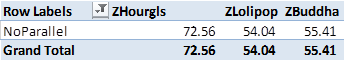
Average time for a full calculation in secs is shown below
One or many
Not shabby as a starting point – both the Lollipop and the Buddha design are significantly faster (around 25%). Interestingly, the site dimension made very little difference to the calculation time, and any other dimensional order was slower. I then started to increase the number of threads available and reran the scripts.
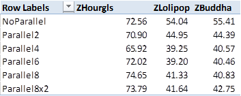
Starting to see some differences. Interestingly, the hourglass design received very little optimisation from parallelism.
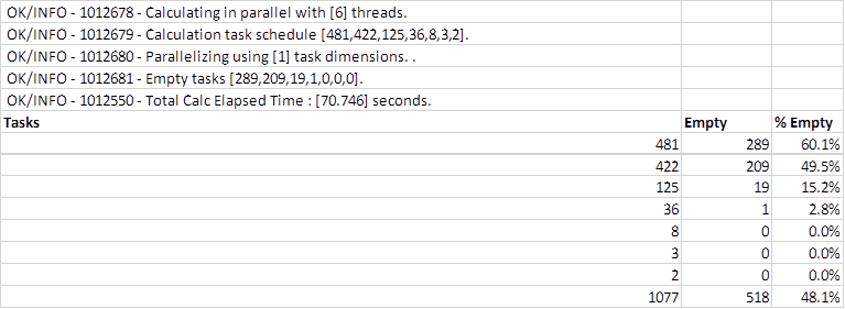
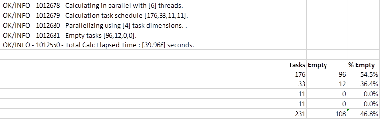
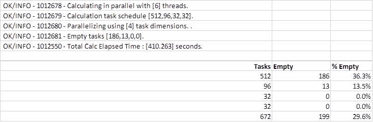
On reviewing the logs, the issue becomes quite apparent – the cost centre dimension is way too sparsely populated to benefit. The first two schedules are greater than 49% empty, and overall the empty tasks are close to 50% of the total tasks. This is due to it only being able to use a single large task dimension (cost centre) to run in –forcing it to use a second dimension as well (expense element) simply makes the performance and emptiness ratio significantly worse.
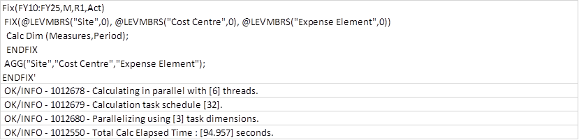
The Lolipop design had a very decent performance bump – and this is caused by a very optimal schedule!
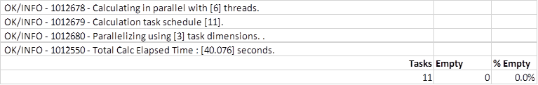
Yep – zero empty tasks. Looking up at the dimensional order it’s easy to work out why. I’m fixing on a single scenario (Rolling) and a single version – so the parallel calculation is running across 11 years (FY15:FY25) – all of which have data. Now, after having a good look through the code, it appears this application ‘can’ calculate years in parallel, however you shouldn’t assume that across all applications. It is very likely that applications carrying balances (ie: BS models, Stock models, physicals models) will either refuse to calculate years in parallel – or will return the wrong values. Testing is important!
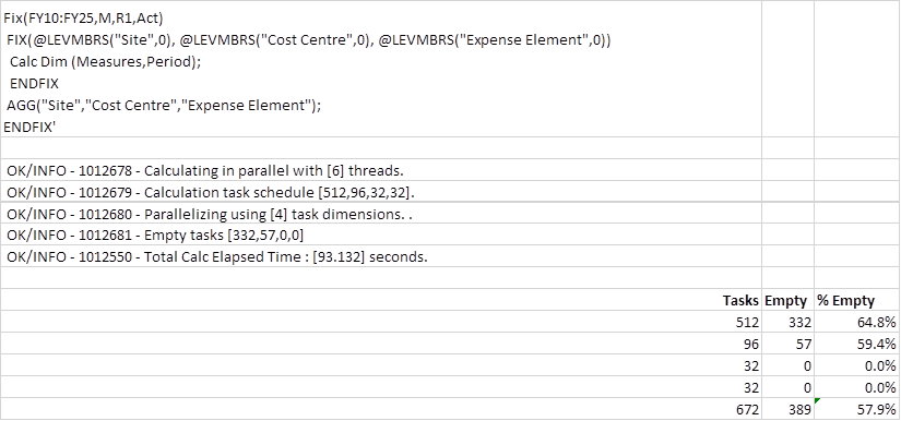
Finally - Buddha.
Very similar performance to the lollipop, but in a slightly different way. It gets the performance optimisation of the Year dimension parallel calc, but the site dimension, while sparse, isn’t big enough to really bog it down. A large number of empty tasks – but it definitely seems that it can handle that without too much of a performance impact if the dimension is smaller.
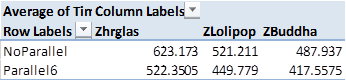
Finally looking back at the calculation times again…there is very little delineation between 2-16 threads. At 2 threads you’ve already picked up 80% of the benefit of parallelisation, and it’s only incremental improvements to a sweet spot of 6 threads. Interestingly, every database was statistically slower when attempting to use anything greater than 8 threads.

Bigger is usually better
Anyways it’s definitely not going to be an interesting article if I leave it here. Let’s crank up the calculations and see if we can force a clear winner between Lollipops and Buddhas. Firstly, let’s increase the fix scope significantly.
Lollipop
Two scenarios, 16 years, 32 scheduled tasks, zero empty tasks. Still very good performance, almost scaling linearly with the fix scope, despite significantly more data in the actual dimension.
Buddha
Similar story, similar outcome. Big increase in the number of tasks, and a greater percentage of empty tasks. Performance is still neck and neck between the two – well within the natural variation of calculations. At this point, I was fairly sure the only way to force delineation between the two would be to artificially increase the density of the Site dimension – so that’s what I did.
Fix(FY10:FY25, R1, Act)
DataCopy Site to PH10;
DataCopy Site to PH20;
DataCopy Site to PH10;
DataCopy Site to PH30;
DataCopy Site to PH90;
DataCopy Site to M00;
DataCopy Site to S6510;
DataCopy Site to E99;
Endfix;
And below is the output.
Overall we’re looking at an 8-10x increase in calculation time pretty much across the board. We’re also seeing Buddha starting to shine…or at least, glimmer faintly.
Buddha
Now the empty ratio is significantly lower and we’re seeing a justifiable performance improvement. That said, the artificial nature in which the Entity dimensions was made more dense isn’t likely to be replicated with a real world data set, so you would definitely need to cherry pick your dimension to get a similar outcome.
Final status- using the Hourglass as our standard.
Row Labels
|
Average of Time
|
Zhrglas
|
100.00%
|
ZLolipop
|
87.33%
|
ZBuddha
|
79.33%
|
Making it easy
Cutting away briefly before delivering the summary. In all of this testing I was finding it very slow having to do the following
- Update a calc script
- Save the calc script
- Run the calc script
- Open the log file
- Find the execution timings of the calc script
- Copy it to a test sheet
- Clear the log file
- Open the calc script again
- Make a minor tweak
- Click save
- Run the script again
- Open the log file etc etc
- Repeat ad nauseum
So I decided to build a method to optimise this a little, setting up a way to grab the information that I needed while making tweaking the calculations a bit more visible. A little known trick is to use MAXL to directly execute calculation commands without the need to create and save calc scripts by making the calculation a string within the MaxL script itself. The format is as follows:
execute calculation
”calc script;”
On App.DB;
This – combined with spooling the output of that calculation to a defined log file means that you can create separate discrete log files for each calculation. For example:
spool on to "d:/Scripts/Parallel/CalcParallel6_ZLolipop_Run1.log";
execute calculation
'SET CALCPARALLEL 6;
Fix(FY10:FY25,M,R1,Act)
FIX(@LEVMBRS("Site",0), @LEVMBRS("Cost Centre",0), @LEVMBRS("Expense Element",0))
Calc Dim (Measures,Period);
ENDFIX
AGG("Site","Cost Centre","Expense Element");
ENDFIX'
on ZLolipop.Costs;
Spool Off;
spool on to "d:/Scripts/Parallel/CalcParallel6_ZHrglas_Run1.log";
execute calculation
'SET CALCPARALLEL 6;
Fix(FY10:FY25,M,R1,Act)
FIX(@LEVMBRS("Site",0), @LEVMBRS("Cost Centre",0), @LEVMBRS("Expense Element",0))
Calc Dim (Measures,Period);
ENDFIX
AGG("Site","Cost Centre","Expense Element");
ENDFIX'
on ZHrglas.Costs;
Spool Off;
Finally – triggering this from a batch script means that we can add a final step (FINDSTR "Elapsed" *.log > CalcTimes.txt) that will scrape all of the Elapsed times and dump them to a central log.
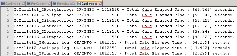
That should help substantially if you wish to run your own test cases!
Pay attention
So what have we learnt from all of this?
- Parallel calculation is a very effective method of gaining a performance boost, and letting Essbase handle most of it using default behaviour works most of the time.
- A lot of this stuff has changed significantly between versions, and what was optimal in 11.1.2.1 (or earlier) is likely not the case now!
- Testing is important
TL;DR Haiku
Lollipops scale better than hourglasses
Buddha on a pole needs a denser bottom
Testing is useful
Pete
Now it’s my turn
What Peter wrote is food for thought, in fact it’s more like a seven course meal. I applaud him for taking the time to figure it out and even more indebted to Peter for writing it all down for world+dog.
I can’t wait to try this out on my next project.
Be seeing you.
1 The problem I’m alluding to is that you’re reading Essbase documentation in the evening rather than socially involving problems like alcoholism
2 Parallel calculations chew a massive amount of ram (as they have the ability to lock out as much as the cache lock setting PER THREAD). Hence, be very cautious being overzealous in Planning scripts where multiple people can run multiple calculations at the same time.
3 I will use the terminology threads and CPUs interchangeably throughout this document. Technically they can’t be interchanged, but my opinion in the matter is near enough is good enough. As a related aside – most of the non-official documentation I’ve read in the last few weeks has suggested that turning Hyper-threading back ON in 11.1.2.3+ environments will actually result in a performance boost.
4 The ‘internal limit’ is an interesting one. It almost seems to hit a complexity limit that cannot be easily bypassed – but as always, documentation on this is sparse. See also SET CALCTASKDIMS for how to increase the number of dims and the complexity level – and generally (in most of my testing) not achieve too much. Essbase does seem to be fairly capable at deciding what will be possible within the guidelines that you give it.
5 That name is all Alan Davey’s fault ladies and gentlemen
6 All calculation times are generally 4-6 runs averaged, removing the major outliers
10 comments:
Superb post, Peter / Cameron. Loads to consider.
"See also SET CALCTASKDIMS for how to increase the number of dims and the complexity level – and generally (in most of my testing) not achieve too much. Essbase does seem to be fairly capable at deciding what will be possible within the guidelines that you give it.". One comment on this - pre 11.1.2.2 (when 'automatic' CALCTASKDIMS arrived) CALCTASKDIMS was always '1' if unspecified, so if your calc FIXed on a single member of the last sparse dimension you'd end up getting no parallelism at all. In a Planning context with (e.g.) Scenario or Fiscal Year last, a good chunk of calcs will run this way. Surprising how often I would see HGOAS recommended *pre*-11.1.2.2 without this caveat.
One other issue I haven't fully got my head around is to what extent the relative 'size' of the tasks matters. For example, if you generate three non-empty tasks and no empty tasks (100% non-empty tasks) but one of those tasks is 100x the size of the other two, I don't think you'll get much benefit from parallelism because the first two threads will sit idle while the third churns. In that situation, increasing CALCTASKDIMS and accepting more empty tasks would likely improve efficiency. The new-ish CALCDIAGNOSTICS logging may help to investigate this further.
These are probably discussions for a beer rather than a blog comment.
Follow-up post could be on how / whether / to what extent FIXPARALLEL changes all this. Can you get that done by the end of the week? :-)
TimG,
Thank you for your kind words but they should be aimed solely at Peter. Okay, you can compliment me for my mysterious ability to trick people into working for me for free in the form of guest posts, but that's all.
As for the rest -- is there anything else you'd like Peter to suss out?
:)
As for the HGOAS approach, we've talked about this before: _knowing_ how something works is different than empirical testing which is different from rules of thumb which is different from "I heard it at a conference so it must be true", all in descending order of usefulness.
Many Essbase/Planning people trend towards the bad end of that spectrum.
And *that's* why the chapters you and Martin wrote for DEA II will be so important -- concepts, design, benchmarking -- these good practices are given their proper due.
Regards,
Cameron Lackpour
P.S. I'd like to think that all of DEA II works through a good practices lens but I think the above two chapters illustrate that the most.
I very interesting post that shows what I knew empirically is in fact accurate. I applaud Peter for taking the time and energy to share this with us. The two tests I would like to see are 1. the same as TimG how FixParallel could be utilized to tweak performance. 2. How an Exalytics X3-4 compares to a X4-4 in parallel calculations. In testing the X3-4 we found after 12- 16 threads performance dedgradated. It is supposed to be fully scalable on the X4-4
Hey Tim,
The size of the task is an interesting point - the testing I did adding in Actuals and future years suggested that the scalability of the parallel calculation is pretty linear. The actual periods are significantly more dense in a data sense (4-5 times maybe? difficult to say for sure). If it was 100x I think you'd definitely have to test it further to see, because I'm inclined to agree that it'll not be as efficient.
FIXPARALLEL is awesome though. Basically, you get to control your empty tasks to quite a detailed level. I'm seeing some major optimisations in allocation type calculations where you're fixing on only items that you want to calculate and which have data. You effectively force reduce the number of empty tasks through fix statements.
It was going to be next on my list (after partitioning, ODI, ASO optimisation and the plethora of other things that are already on it...)
Finally, CALCDIAGNOSTICS is very useful for identifying optimal calculations - unfortunately the format of it sucks pretty badly if you want to do a lot of testing. I've ended up scripting to dodgy batch parsing to grab those lines and break them up.
Also - HGOAS?
Thanks for your comments, Peter. HGOAS = "Hourglass on a stick" :-)
@GlennS, I believe the X4-4 being more scalable is more a function of 11.1.2.4 versus the hardware. Suggest you will see 11.1.2.4 on X3-4 improve scaling per the updated "Secret Sauce". The higher load scaling better is due to updates to the locking mechanisms used in software which should be supported across the whole Exalytics family.
Kind Regards,
John
@John A. Booth, I agree scalability is a factor of the software, but since the X4-4 also has optimizations on the chip to shut off chips not in use and speed up those chips being used, there might be some additional bump because of that. testing the X3 vs the X4 would prove or disprove that at different levels of parallalism
Great information, Test Data in Software Testing have high importance while doing data driven testing or generating databases.
Hi guys. Love this stuff. Since 11.1.2.3.500 is mentioned as the latest release for the article, I suggest this: use FixParallel to change the task dims used for parallelism without having to change outline order. This is the main reason we implemented FixParallel. I find that with fixes on these lollipop dims at the bottom of the outline, it can cause a multiplied effect when it reaches the "large" task dimension. For example: one scenario, one version, one year etc. and then a large sparse dim you are fine for CalcParallel. It will make tasks from the large dim. But if you have two scenarios, one version, two years; then 4 tasks is generally too few and 4x that large spase dim is too many. FixParallel is the way to go when CP can't do it with your proven outline order. No reason to change the outline.
Post a Comment