Cell Text exposure to OBI

Yr. Obt. Svt.’s introduction

I have yet again managed to sucker convince a guest writer, in this case Igor Slutskiy to do my work for me share valuable information with you, Gentle Reader.

This post is a bit unusual in that it targets OBIEE but I’ve been remiss in not covering, or trying to cover, OBI.  Happily Igor has taken that off my hands.  

I’ll also note that while many of us are not OBI geeks, the techniques Igor shows below allows Cell Text (and other index-based Planning repository data) to be viewed within any relational tool and it also shows how to take fact data and create a star schema from it.  Fully (or almost fully) normalized tables rule!

Also, I should note that this approach shows how to take a periods across the columns table and convert it to one that places periods down with a single fact column.  Glenn aka MMIC just wrote about one approach to do this but I like this one better.   The below technique is predicated on using a relational target, but we should be doing everything in SQL, right?  Death to flat files!

With that, let Igor take it away.

The Issue

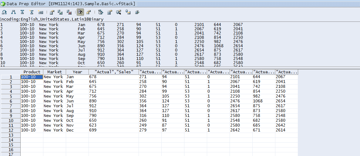
Cell Text (CT) is a functionality of Planning that allows storing text in a cell.  In the picture below, the first 2 columns store text and the next column stores values.  In order to store text, a member has to be setup with a “Text” data type.    

Essbase can store only values, so Planning creates a numerical index for a text item and stores it in Essbase, while storing the actual text in the Relational Database (RDB).  The table in RDB has only 2 columns:  the CT and the numerical index for it.  OBI can connect to Essbase, but it would only retrieve a numerical index, as CT is not stored there.  OBI can also connect to RDB, but RDB does not store metadata for the CT items.  

The Solution

Bring metadata for the CT items into RDB and use the same approach to retrieve CT as is used for Cell Notes retrieval.  Here are the steps:

1. Create a table in RDB that will contain metadata and the numerical index for CT.  We can bring the content will come from Essbase.
2. Define a data set with text members in Essbase.
3. Export the above data set from Essbase into RDB table created earlier.
4. Reconstruct the RDB table into a star-schema compatible table.
5. Create dimensional tables and a fact table for a complete star-schema.
6. OBI connects to the star-schema in RDB, joins to Essbase and retrieves CT.

NOTE1:  the solution may be changed to use a single table in step 1 and using views instead of other tables.  Views typically perform slower than tables.  Performance could be tested and a decision on the method would be finalized.  

NOTE2:  the tables/views would be created in the Planning schema.

NOTE3:  all processes can be scripted and automated.

Refer to the flowchart below as you read this design document.

T_CELL_TEXT_ESSBASE_DATA

T_CELL_TEXT_DATA

 T_CELL_TEXT_FACT

HSP_TEXT_CELL_VALUE

Solution Steps

Create a table in RDB that will contain metadata and the numerical index for CT

Essbase exports data in the following format:  1 column for each dimension except for a Period dimension; 1 column for each Period dimension.  For example, if we have a total of 12 dimensions and want to export Level 0 periods, we will have a total of 23 columns (11 columns for each dimension except for a Period dimension plus 12 columns for Jan-Dec periods).

A table T_CELL_TEXT_ESSBASE_DATA is created:

-- 1. CREATE A TABLE TO TAKE THE IMPORT FROM ESSBASE (ONE TIME EVENT)

 DROP TABLE T_CELL_TEXT_ESSBASE_DATA;

CREATE TABLE T_CELL_TEXT_ESSBASE_DATA

  (

    "YEAR" VARCHAR2(255 CHAR),

    "SCENARIO" VARCHAR2(255 CHAR),

    "VERSION" VARCHAR2(255 CHAR),

    "ENTITY" VARCHAR2(255 CHAR),

    "DATATYPE" VARCHAR2(255 CHAR),

    "LEDGER" VARCHAR2(255 CHAR),

    "PRODUCT" VARCHAR2(255 CHAR),

    "SEGMENT" VARCHAR2(255 CHAR),

    "SOURCE" VARCHAR2(255 CHAR),

    "CURRENCY" VARCHAR2(255 CHAR),

    "ACCOUNT" VARCHAR2(255 CHAR),

    "JAN" NUMBER(*,0),

    "FEB" NUMBER(*,0),

    "MAR" NUMBER(*,0),

    "APR" NUMBER(*,0),

    "MAY" NUMBER(*,0),

    "JUN" NUMBER(*,0),

    "JUL" NUMBER(*,0),

    "AUG" NUMBER(*,0),

    "SEP" NUMBER(*,0),

    "OCT" NUMBER(*,0),

    "NOV" NUMBER(*,0),

    "DEC" NUMBER(*,0)

  );

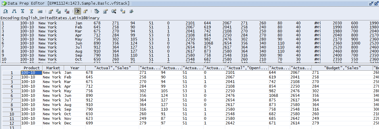
The resulting table contains a numerical index of the Cell Text in each Period column:

Define a data set with text members in Essbase

For POC the following data set has been defined which mainly corresponds to the screenshot in The Issue section:

   

@RELATIVE("YearTotal",0),@DESCENDANTS("Source "), "Actual", "Working", "Amount", "GAAP", "Product 1", @DESCENDANTS("Accounts"), "Company 1", "SEG 1", "USD", "FY10"

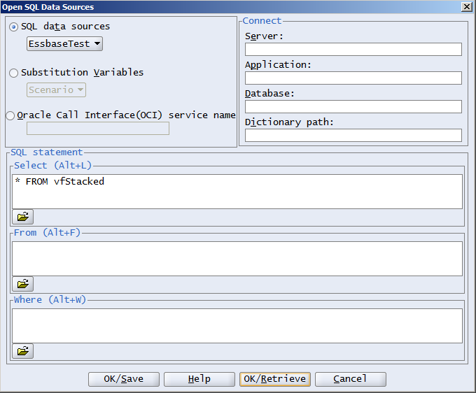
Export the data set from Essbase directly into RDB

A script is created to accomplish this task:

Name:          Exp_CellText_Level0.mxls

Location:    /opt/app/hyp/batch/maxl/

Code:        the code below is included inside a wrapper

SET DATAEXPORTOPTIONS

{

DataExportLevel "LEVEL0";

DataExportRelationalFile ON;

DATAEXPORTOVERWRITEFILE ON;

};

FIX (@RELATIVE("YearTotal",0),@DESCENDANTS("Source"), "Actual", "Working", "Amount", "GAAP", "Product 1", @DESCENDANTS("Accounts "), "Company 1", "SEG 1", "USD", "FY10");

   DATAEXPORT "DSN" "dsn_name" "T_CELL_TEXT_ESSBASE_DATA" "schema" "password";

ENDFIX;

Reconstruct the RDB table into a star-schema compatible table.

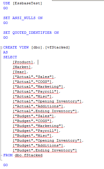
The following code creates a T_CELL_TEXT_DATA table which is reconstructed from T_CELL_TEXT_ESSBASE_DATA to a star-schema compatible format.  Note, this table is constructed for the quarter-end months, to reflect the current reporting practices.  This script includes quarter-end periods, but could be easily modified to include additional periods.

  

-- 2. CREATE A SINGLE-MEASURE COLUMN TABLE FROM THE ABOVE (PERIODIC UPDATE).

 DROP TABLE T_CELL_TEXT_DATA;

CREATE TABLE T_CELL_TEXT_DATA AS

SELECT

 'Mar' AS "PERIOD",

 "YEAR", "SCENARIO", "VERSION", "ENTITY", "DATATYPE", "LEDGER", "PRODUCT", "SEGMENT", "SOURCE", "CURRENCY", "ACCOUNT",

 "MAR" AS TEXT_ID

FROM T_CELL_TEXT_ESSBASE_DATA

  UNION ALL

SELECT

 'Jun' AS "PERIOD",

 "YEAR", "SCENARIO", "VERSION", "ENTITY", "DATATYPE", "LEDGER", "PRODUCT", "SEGMENT", "SOURCE", "CURRENCY", "ACCOUNT",

 "JUN" AS TEXT_ID

FROM T_CELL_TEXT_ESSBASE_DATA

  UNION ALL

SELECT

 'Sep' AS "PERIOD",

 "YEAR", "SCENARIO", "VERSION", "ENTITY", "DATATYPE", "LEDGER", "PRODUCT", "SEGMENT", "SOURCE", "CURRENCY", "ACCOUNT",

 "SEP" AS TEXT_ID

FROM T_CELL_TEXT_ESSBASE_DATA

  UNION ALL

SELECT

 'Dec' AS "PERIOD",

 "YEAR", "SCENARIO", "VERSION", "ENTITY", "DATATYPE", "LEDGER", "PRODUCT", "SEGMENT", "SOURCE", "CURRENCY", "ACCOUNT",

 "DEC" AS TEXT_ID

FROM T_CELL_TEXT_ESSBASE_DATA ;

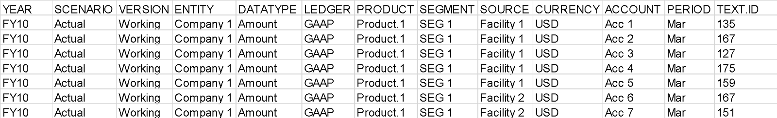
The restructured table above T_CELL_TEXT_DATA is different from the T_CELL_TEXT_ESSBASE_DATA table in that it establishes an additional column for the Period dimension and pivots the Period columns (Jan-Dec) into rows, leaving a single value column labeled TEXT_ID.  This is the column that holds the numeric index of the CT items.

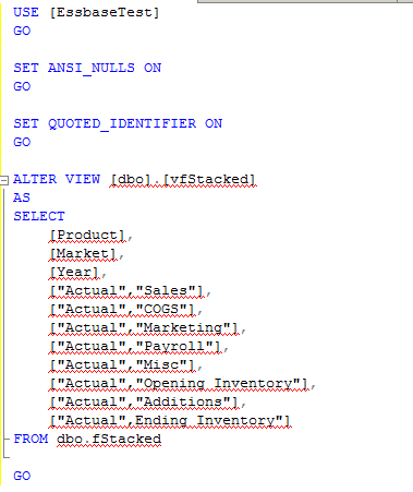
Create star-schema tables

The T_CELL_TEXT_DATA table will be used as a basis to create the star-schema tables required for OBI – 1 fact table and 12 dimension tables.

Create a Fact Table

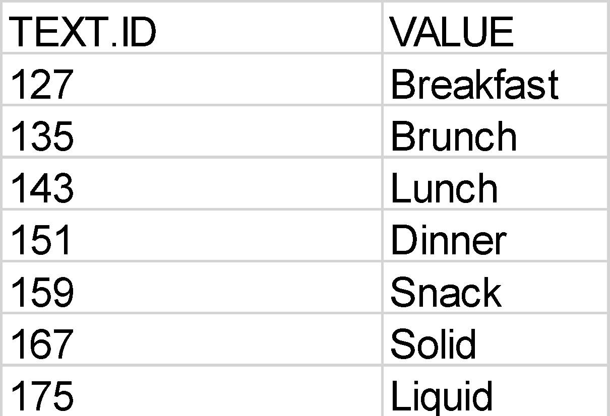
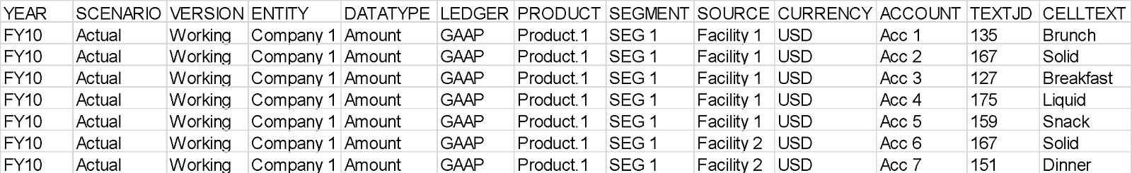
To get CT, T_CELL_TEXT_DATA table will be joined to HSP_TEXT_CELL_VALUE, a Planning native table that holds CT and its numeric index.  The 2 tables will be joined by the numeric index (TEXT_ID) creating the T_CELL_TEXT_FACT table.

-- 3. CREATE A FACT TABLE BY JOINING THE ABOVE TABLE TO HSP_TEXT_CELL_VALUE (PERIODIC UPDATE).

 DROP TABLE T_CELL_TEXT_FACT;

CREATE TABLE T_CELL_TEXT_FACT AS

 SELECT T_CELL_TEXT_DATA.*, HSP_TEXT_CELL_VALUE.VALUE AS CELLTEXT

 FROM T_CELL_TEXT_DATA

 INNER JOIN HSP_TEXT_CELL_VALUE

 ON T_CELL_TEXT_DATA.TEXT_ID = HSP_TEXT_CELL_VALUE.TEXT_ID;

Here is the Planning native HSP_TEXT_CELL_VALUE table:

Note a new CELLTEXT column in the resulting T_CELL_TEXT_FACT table.

Create dimensional tables

The following code creates T_CELL_TEXT_DIM_* dimension tables where * denotes a dimension name.

-- 4. CREATE DIMENSION TABLES (PERIODIC UPDATE).

 DROP TABLE T_CELL_TEXT_DIM_PERIOD;

CREATE TABLE T_CELL_TEXT_DIM_PERIOD AS

 SELECT DISTINCT "PERIOD"

 FROM T_CELL_TEXT_DATA;

 

 DROP TABLE T_CELL_TEXT_DIM_YEAR;

CREATE TABLE T_CELL_TEXT_DIM_YEAR AS

 SELECT DISTINCT "YEAR"

 FROM T_CELL_TEXT_DATA;

 

 DROP TABLE T_CELL_TEXT_DIM_SCENARIO;

CREATE TABLE T_CELL_TEXT_DIM_SCENARIO AS

 SELECT DISTINCT "SCENARIO"

 FROM T_CELL_TEXT_DATA;

 

 DROP TABLE T_CELL_TEXT_DIM_VERSION;

CREATE TABLE T_CELL_TEXT_DIM_VERSION AS

 SELECT DISTINCT "VERSION"

 FROM T_CELL_TEXT_DATA;

 

 DROP TABLE T_CELL_TEXT_DIM_ENTITY;

CREATE TABLE T_CELL_TEXT_DIM_ENTITY AS

 SELECT DISTINCT "ENTITY"

 FROM T_CELL_TEXT_DATA;

 

 DROP TABLE T_CELL_TEXT_DIM_DATATYPE;

CREATE TABLE T_CELL_TEXT_DIM_DATATYPE AS

 SELECT DISTINCT "DATATYPE"

 FROM T_CELL_TEXT_DATA;

 

 DROP TABLE T_CELL_TEXT_DIM_LEDGER;

CREATE TABLE T_CELL_TEXT_DIM_LEDGER AS

 SELECT DISTINCT "LEDGER"

 FROM T_CELL_TEXT_DATA;

 

 DROP TABLE T_CELL_TEXT_DIM_PRODUCT;

CREATE TABLE T_CELL_TEXT_DIM_PRODUCT AS

 SELECT DISTINCT "PRODUCT"

 FROM T_CELL_TEXT_DATA;

 

 DROP TABLE T_CELL_TEXT_DIM_SEGMENT;

CREATE TABLE T_CELL_TEXT_DIM_SEGMENT AS

 SELECT DISTINCT "SEGMENT"

 FROM T_CELL_TEXT_DATA;

 

 DROP TABLE T_CELL_TEXT_DIM_SOURCE;

CREATE TABLE T_CELL_TEXT_DIM_SOURCE AS

 SELECT DISTINCT "SOURCE"

 FROM T_CELL_TEXT_DATA;

 

 DROP TABLE T_CELL_TEXT_DIM_CURRENCY;

CREATE TABLE T_CELL_TEXT_DIM_CURRENCY AS

 SELECT DISTINCT "CURRENCY"

 FROM T_CELL_TEXT_DATA;

 

 DROP TABLE T_CELL_TEXT_DIM_ACCOUNT;

CREATE TABLE T_CELL_TEXT_DIM_ACCOUNT AS

 SELECT DISTINCT "ACCOUNT"

 FROM T_CELL_TEXT_DATA;

 

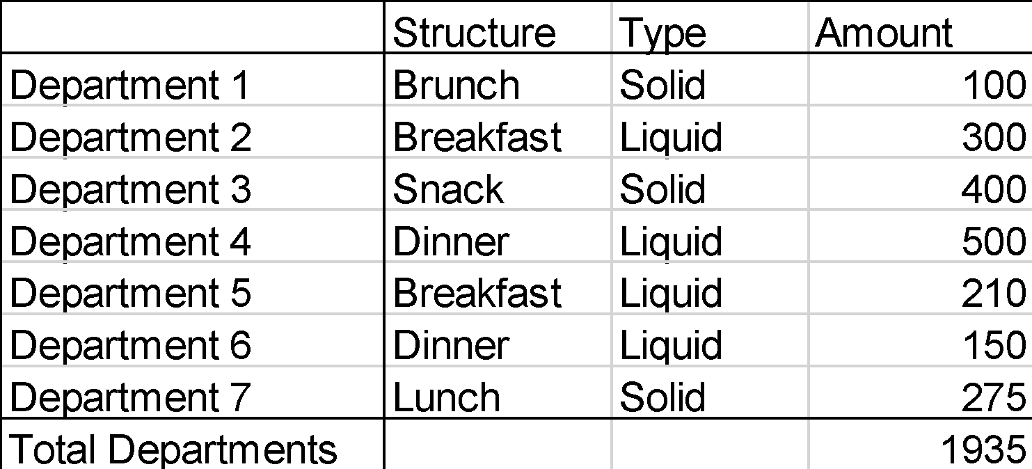
Here is an example of the resulting ACCOUNT dimension table:

Summary

In the above example, fifteen tables are created:

1 for Essbase Data

1 for Conversion

1 for Facts

12 for each Dimension

As noted above, all tables except for the Essbase Data table could be substituted with Views.

All processes above could be scripted and completely automated.

Yr. Obt. Svt’s conclusion

Igor, again my thanks for writing this.  There’s more to life than just Planning and Essbase (although those are the products that Keep Cameron Housed) and many Oracle EPM folks use OBI.  Hopefully this post will be one in a series of OBI/EPM posts.

Having written that, I’m making an appeal to you, oh Best and Brightest:  if you are an OBI/EPM geek, and you want to see your name in print, please contact me (you likely know my email address from Kscope, OOW, etc. or via LinkedIn) and I’ll give you a post or more if you’re really enthusiastic.  This site gets around 9,000 page views and about 7,000 sessions so you’ll have an audience.  

This offer goes out to all interested writers, OBI geek or otherwise.  The purpose of this blog is to share information.  I’m happy to provide the medium to do so.

Be seeing you.

Stupid Programming Tricks No 29, part 2 -- Dynamic Load Rule columns

Where we were or where are  we or most importantly where am I?

I have no idea as to the last point but then again I never do.  Ever.

Moving on, in the first part of this exciting (surely not but at least useful) series, I related how to stack dimensions in a single column.

Alas and alack, My Man In California, Glenn Schwartzberg, pointed out in the comments to that post that he had already covered this at two different Kscopes.  Oh the shame, but as a soon-to-be-ex-board member the number of sessions I get to attend is severely limited.  Sorry, Glenn.  I had to figure it out on my own.  I never do things the easy way.  Ever.  Again.  Bugger.

The Network54 use case I addressed was primarily a need to both stack dimensionality as well as selectively address more or fewer columns of data depending on data scope.

This is quite easily done in a Load Rule, indeed it’s possible in both a SQL as well as text Load Rule and it all centers around how the initial record of a Load Rule.  The Stupid Trick here is that if ten data columns are defined at design-time and only five are passed at load time, the Load Rule ignores the last five.

One might think that this would be best accomplished by changing the SQL query within the Load Rule but by doing that one would edit the Load Rule itself, this would be a design-time change , and the number of columns would be modified.  I’ll also mention that Load Rules are tricky little buggers that just beg to go FOOM! so I’m loathe to modify them.  

Instead, a SQL view that changes the scope of the columns passed to the Load Rule’s SELECT (well, you have to skip the “SELECT” but that’s the action the rule performs) * FROM viewname and ta-da, the Load Rule now selects fewer (or even more with an important caveat) data columns.

That caveat

This more-or-less Load Rule behavior is predicated on the columns that are defined within a SQL view.

I take the point, perhaps even before you’ve raised it, that modifying the SQL is a design-time change.  But with these requirements something and somehow is going to change.  Load Rule or ALTER VIEW?  One man’s meat is another man’s poison so it’s time to pick yours.

What kind of poison for the evening, sir?

I’ll have just a wee slice of SQL:

Pulling this in a SQL Load Rule looks like this:

And this:

So no different than the original fStacked table which is in turn no surprise given that the fields are the same in the view as they are in the table.

Let’s cut that view down to just Actual columns:

Et voilà!, dynamic Load Rules

Change the SQL in the view, no change to the rule, change the data columns and thus scope, all with no editing of The Devil’s Own.  Gee whiz, could it be that Load Rules aren’t spawn from Old Scratch?  Maybe.

Would I do it this way?

Let’s review what this approach does:

• It stacks dimensions in a column, i.e. it allows more than one dimension to be defined for each column of fact data.  That’s not a condition of dynamic Load Rules but instead is a requirement of that post way back when in part 1.
• It shows that removing or adding columns to a data source make the Load Rule display more or fewer columns.

The caveat to the above approach is that the definition of the Load Rule’s columns must happen before the data change and the maximum number of possible columns needs to be defined up front.  

If this last bit seems odd, think what happens when you load a poorly defined text file such as when you’re told, “There are 13 columns of data,” but in fact there’re really 14 columns 2,312 records down although not in the first 2,311 rows.  Whoops, someone forgot to mention that and because the Load Rule defines columns based on its initial 50 row read (yes, you can change this and even the starting position but you’d have to know the exact row to go to) Essbase is going to throw a rod because it doesn’t know how to handle data column 14.  The damnable thing of it is if the Load Rule can’t see the column, the Essbase geek can’t add it.  The “fix” is to create a one record file that has that 14th column, tag the column as Ignore During Data Load, and for the 2,311 preceding rows it’s as if that column doesn’t exist (remember there is no tab or comma delimiter at the end of those 13 fact field records) until record 2,312.  This is the same concept as the “Budget”,”Sales” columns defined when the data exists and then being dropped when the data source no longer contains said columns.

Whew.

So what do I do?  Benchmark.  I’d benchmark this approach, particularly the full Actual and Budget load example vs. two separate Load Rule streams, one of Actual and the other of Budget.  And as this is an ASO cube, I’d kick that latter approach off in multiple MaxL statements writing the contents to a single buffer.  Is the performance issue tied to how fast Essbase can commit a temporary tablespace to a permanent one or is it how big the pipe from the fact source is?  Dunno till tested.  

If a two stream approach worked, there’d need to be some kind of conditional branching in the batch script to decide which or both to load.  

Whew, again.  No one said that system requirements are easy.  That’s why we’re (hopefully) paid the big (even more hopefully) bucks (insert currency of your choice).

Be seeing you.